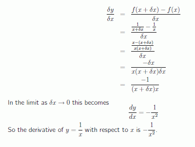
Differentiation From First Principles

This section looks at calculus and differentiation from first principles.

Differentiating a linear function

A straight line has a constant gradient, or in other words, the rate of change of y with respect to x is a constant.

Example

Consider the straight line y = 3x + 2 shown below

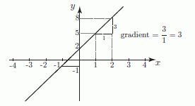
A graph of the straight line y = 3x + 2.

We can calculate the gradient of this line as follows. We take two points and calculate the change in y divided by the change in x.

When x changes from −1 to 0, y changes from −1 to 2, and so

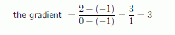
No matter which pair of points we choose the value of the gradient is always 3.

Values of the function y = 3x + 2 are shown below

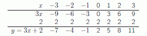
Look at the table of values and note that for every unit increase in x we always get an increase of 3 units in y. In other words, y increases as a rate of 3 units, for every unit increase in x. We say that “the rate of change of y with respect to x is 3”.

Observe that the gradient of the straight line is the same as the rate of change of y with respect to x.

NOTE: For a straight line: the rate of change of y with respect to x is the same as the gradient of the line.

Differentiation from first principles of some simple curves

For any curve it is clear that if we choose two points and join them, this produces a straight line.

For different pairs of points we will get different lines, with very different gradients. We illustrate below.

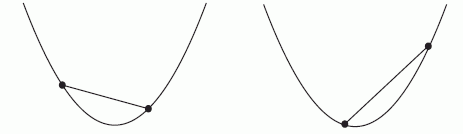
Joining different pairs of points on a curve produces lines with different gradients

Example : Suppose we look at y = x².

Note that as x increases by one unit, from −3 to −2, the value of y decreases from 9 to 4. It has reduced by 5 units. But when x increases from −2 to −1, y decreases from 4 to 1. It has reduced by 3. So even for a simple function like y = x² we see that y is not changing constantly with x. The rate of change of y with respect to x is not a constant.

Calculating the rate of change at a point

We now explain how to calculate the rate of change at any point on a curve y = f(x). This is defined to be the gradient of the tangent drawn at that point as shown below

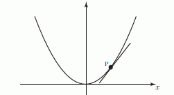
The rate of change at a point P is defined to be the gradient of the tangent at P.

NOTE: The gradient of a curve y = f(x) at a given point is defined to be the gradient of the tangent at that point.

We use this definition to calculate the gradient at any particular point.

Consider the graph below which shows a fixed point P on a curve. We also show a sequence of points Q1, Q2, . . . getting closer and closer to P. We see that the lines from P to each of the Q’s get nearer and nearer to becoming a tangent at P as the Q’s get nearer to P.

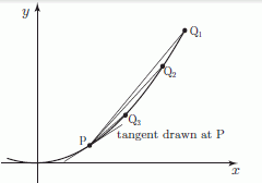
The lines through P and Q approach the tangent at P when Q is very close to P.

So if we calculate the gradient of one of these lines, and let the point Q approach the point P along the curve, then the gradient of the line should approach the gradient of the tangent at P, and hence the gradient of the curve.

Example : We shall perform the calculation for the curve y = x² at the point, P, where x = 3.

The graph below shows the graph of y = x² with the point P marked. We choose a nearby point Q and join P and Q with a straight line. We will choose Q so that it is quite close to P. Point R is vertically below Q, at the same height as point P, so that △PQR is right-angled.

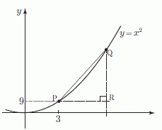
The graph of y = x². P is the point (3, 9). Q is a nearby point.

Suppose we choose point Q so that PR = 0.1. The x coordinate of Q is then 3.1 and its y coordinate is 3.1². Knowing these values we can calculate the change in y divided by the change in x and hence the gradient of the line PQ.

We can take the gradient of PQ as an approximation to the gradient of the tangent at P, and hence the rate of change of y with respect to x at the point P.

The gradient of PQ will be a better approximation if we take Q closer to P. The table below shows the effect of reducing PR successively, and recalculating the gradient.

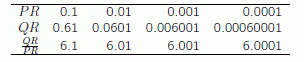
The gradient of the line PQ, QR/PR seems to approach 6 as Q approaches P.

Observe that as Q gets closer to P the gradient of PQ seems to be getting nearer and nearer to 6.

We will now repeat the calculation for a general point P which has coordinates (x, y).

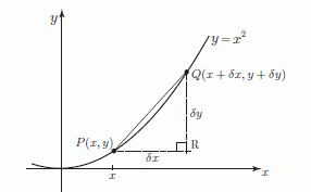
The graph of y = x². P is the point (x, y). Q is a nearby point.

Point Q is chosen to be close to P on the curve. The x coordinate of Q is x + dx where dx is the symbol we use for a small change, or small increment in x. The corresponding change in y is written as dy. So the coordinates of Q are (x + dx, y + dy).

Because we are considering the graph of y = x², we know that y + dy = (x + dx)².

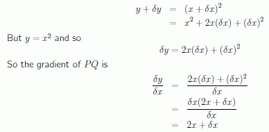
As we let dx become zero we are left with just 2x, and this is the formula for the gradient of the tangent at P. We have a concise way of expressing the fact that we are letting dx approach zero. We write

‘lim’ stands for ‘limit ’and we say that the limit, as x tends to zero, of 2x+dx is 2x. Note that when x has the value 3, 2x has the value 6, and so this general result agrees with the earlier result when we calculated the gradient at the point P(3, 9).

We can do this calculation in the same way for lots of curves. We have a special symbol for the phrase

We write this as dy/dx and say this as “dee y by dee x”. This is also referred to as the derivative of y with respect to x.

Use of function notation

We often use function notation y = f(x). Then, the point P has coordinates (x, f(x)). Point Q has coordinates (x + dx, f(x + dx)).

So, the change in y, that is dy is f(x + dx) − f(x). Then,

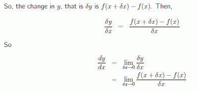
This is the definition, for any function y = f(x), of the derivative, dy/dx

NOTE: Given y = f(x), its derivative, or rate of change of y with respect to x is defined as

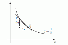
Example

Suppose we want to differentiate the function f(x) = 1/x from first principles.

A sketch of part of this graph shown below. We have marked point P(x, f(x)) and the neighbouring point Q(x + dx, f(x +d x)).

Differentiation From First Principles

Log in